The art of finding transition structures

Finding transition structures is one of the most challenging tasks in computational organic chemistry; moreso than ground state optimizations since the resulting structures are, by definition, unstable ones. The process requires both careful setup of the problem as well as the dreaded chemical intuition.

This lesson will focus on four methods of searching for transition structures. They will be presented in descending order of utility (i.e. the most likely to work to the least likely to work). Which means that you, dear user, should try this list from top to bottom.

2-Structure Synchronous Transit-Guided Quasi-Newton Method (QST2)
TS guess with frozen bond approximations
3-Structure Synchronous Transit-Guided Quasi-Newton Method (QST3)
Relaxed potential energy scan

2-Structure Synchronous Transit-Guided Quasi-Newton Method (QST2)

The Synchronous Transit-Guided Quasi-Newton methods were developed by Peng and Schlegel in the 90s.¹ These methods employ a linear or quatradic synchronous transit (L/Q-ST) approach to approximate the saddle region and then switch to a quasi-Newton search for the true transition structure. In a the synchronous transit approach a (linear or parabolic) path along the reaction coordinates is plotted and the energies along the path are sampled (Fgiure 1a). The highest energy structure along the path is then efficiently optimized to the transition structure (Figure 1b) using an approximate quadratic search (quasi-Newton).

Figure 1. a| Linear (LST) and quadratic (QST) synchronous transit paths.
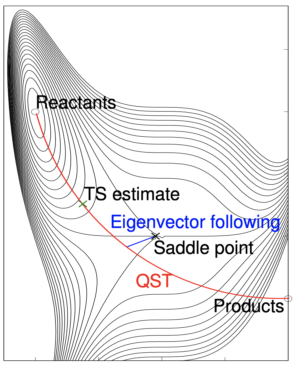
b| Eigenvector search from QST maximum to the saddle point. Reproduced from ref 2.

To set up a QST2 calculation you’ll need two structures:

The reactant ensemble
The product ensemble

I call these ensembles because (unless you’re studying a unimolecular to unimolecular reaction) these starting geometries will comprise of multiple fragments. They should be fully optimized; sometimes this requires a bit of fine tuning since Gaussian may want to kick off one of the reactants to make a more favorable “molecule”, but persistence is key in this step. After optimizing the reactant and product ensembles you’ll submit a Gaussian input with the following format:

%chk=jobName.chk     ! you want to save a checkpoint, can also do this with GAUSS_YDEF
#N M062X/def2svp OPT=QST2 Freq=(NoRaman) ...    ! all optimizations need a freq
<<Blank line>>       ! QST2 tells g16 that we want a transition structure search
Reactants title section
<<Blank line>>
Molecule specification for the reactants
<<Blank line>>
Products title section
<<Blank line>>
Molecule specification for the products
<<Blank line>>       ! additional input, if any, follows
...

The atom numbers in both molecule specifications must be the same so that Gaussian can map the reaction coordinate atom by atom.

The starting guess for the transition structure is midway between the reactant and product geometries, which is why these structures must be optimized beforehand. Additionally, this allows you to calculate a $\Delta G^{\ddagger}_{rxn}$. In Gaussian the QST2 is the quickest path to a saddle point and typically works well. However, this method fails if the “average” geometry between reactants and products is chemically illogical (e.g., complex stereoinversions and isomerizations). For example, consider the isomerization of hydrogen cyanide to hydrogen isocyanide (Figure 2). In this case the “average” structure places the hydrogen inside the C≡N bond. A QST2 search of this reaction will not converge to the true three-center transition structure.

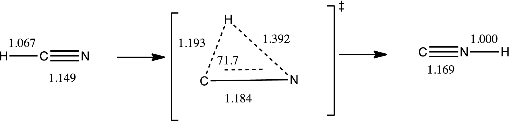Figure 2. The isomerization of isomerization of hydrogen cyanide to hydrogen isocyanide. Reproduced from ref. 3.

If your calculation converges to a logical transition structure skip down to the verification section. If your calculation has trouble converging to a stationary point you can try adding calculating force constants at the start of the optimization with OPT=(QST2,calcFC). This will add a small amount of time, but will ensure that the optimization gets started correctly. The option calcFC calculates force constants for the first step in the optimization; use calcALL to tell Gaussian to calculate force constants at every step of the optimization. N.b. this is only for very difficult convergence issues and will add a significant amount of time to your calculation; if you’re considering this option seek help first as there’s probably a unseen issue that’s causing your jobs to fail. If this method won’t work for you, try a TS guess!

TS guess with frozen bond approximations

So the QST2 didn’t work (either because it failed or the algorithm didn’t find the correct structure). This next method has two parts:

Build a model of the most likely transition structure (this is where you chemical intuition is needed) and optimize all the atoms that don’t participate in the reaction.
Re-optimize the transition structure now with all atoms free.

One could ask, why we’re not trying the QST3 method mentioned below. QST3 requires a “best guess” on the transition structure, which is what we’ll make in the first step of this method. So if we’ll need to partially optimize a best guess anyways, we might as well attempt a direct optimization of the transition structure.

Keep in mind, designing a transition structure by hand is no trivial task; bond lengths, angles, and dihedrals are all significant factors. Furthermore, the saddle point you find is sensitive to the initial guess. Whether or not you correctly identify the true saddle structure is wholely dependent on whether or not you start with the correct geometry.

A transition structure search is called using the keyword OPT=TS, we’ll also use the additional options to help guide the calculation to convergence:

CalcFC: Calculates the force constants for the first structure
NoEigenTest: Suppresses testing of the eigenvalues during the optimization (common cause of failure)
ModRedundant/AddGIC: Allows us to freeze bond lengths/positions during the optimization

%chk=jobName.chk     ! you want to save a checkpoint, can also do this with GAUSS_YDEF
#N M062X/def2svp OPT=(TS,CalcFC,NoEigenTest,AddGIC/ModRedundant) ...
<<Blank line>>
Title section
<<Blank line>>
Molecule specification
<<Blank line>>
Coordinates of active atoms
<<Blank line>>       ! additional input, if any, follows
...

At the end of this first optimization you’ll need to tell Gaussian which bonds to freeze during the optimization. If you’re optimizing using Gaussian’s redundant internal coordinates (the default) then this last section will take the form: B [Atom 1 number] [Atom 2 number] F where atoms 1 and 2 will be frozen in the geometry optimization. For example, B 74 94 F freezes the bond (length and position) between atom 74 and 94.

If you’re optimizing using the new Generalized Internal Coordinates (GICs) the section will look like: CoordinateName(freeze)=R(Atom 1 number,atom 2 number) where atoms 1 and 2 will be frozen in the geometry optimization. For example, BrC(freeze)=R(74,94) freezes the coordinate between atoms 74 and 94. In this method each frozen coordinate must have its own unique name.

Once the optimization has converged (if it does converges, see note below), reoptimize the structure using the same routing line, but without AddGIC/ModRedundant and the coordinate section at the end. Don’t forget to add a freq calculation!

N.b. This optimization may not converge, sometimes the first step doesn’t end up finding a true minimum because the frozen coordinates are frozen in such a way that they prevent the convergence criteria from being met. You have to keep an eye on these calculations in case they end up oscillating between two similar structures. If this happens, just cancel the job and use one of these structures as the starting point for the next optimization.

If this calculation converges then skip down to the verification section. Of course, there’s always the possibility that the molecule relaxes down to the product or reactant geometries at this stage (this happens more often than you’d like). This is typically an indicator that your initial transition state guess is incorrect. In this case, start from the result of the first optimization step and tweak the active atoms (bond lengths, angles, etc…) in the starting geometry for the second optimization. This method can be fickle, but when it does work it’s quite elegant. If you’ve tried several times and still have no luck, proceed to the QST3 method in the next section.

3-Structure Synchronous Transit-Guided Quasi-Newton Method (QST3)

The QST3 method uses the same search algorithm as QST2, but takes one more input: a “best guess” or ansatz of your transition structure. The quadratic synchronous transit then draws a parabolic search path from the reactants to the products through the ansatz in the reaction coordinate space and then proceeds in the same manner as a QST2 search.

To call the QST3 search in Gaussian use the OPT=QST3 keyword:

%chk=jobName.chk     ! you want to save a checkpoint, can also do this with GAUSS_YDEF
#N M062X/def2svp OPT=QST3 Freq=(NoRaman) ...    ! all optimizations need a freq
<<Blank line>>       ! QST3 tells g16 that we want a transition structure search
Reactant title section
<<Blank line>>
Molecule specification for the reactants 
<<Blank line>>
Product title section
<<Blank line>>
Molecule specification for the products
<<Blank line>>
Ansatz title section
<<Blank line>>
Molecule specification for the ansatz
<<Blank line>>       ! additional input, if any, follows
...

As in QST2, it is essential that all of the atoms in the molecule specifications are numbered the same. Otherwise, Gaussian won’t be able to correctly map the atoms in the reaction coordinate space. Likewise, the options calcFC and calcALL can help with difficult convergence issues in this calculation. If this calculation converges then skip down to the verification section, otherwise proceed to a potential energy scan.

Potential energy surface scan

If you’ve gotten to this point then we’re really at our wits end. A scan of the potential energy surface essentially implements a linear transit of the specified coordinate calculating the energies of the intermediate structures. Ideally,this method produces an approximation of the reaction pathway along a single reaction coordinate. There are two different kinds of potential energy surface scans available in Gaussian. The rigid potential energy surface scan and the relaxed potential energy scan. A relaxed PES scan optimizes the structures around the specified coordinate values at each step, while a rigid PES scan calculates only energies using the specified coordinates. Both methods work in the same way, but the PES is typically faster (since there are no optimizations to complete), however the result of a rigid PES scan must be reoptimized using the OP=TS method described above. In practice it is good to do the PES scan at a lower (less expensive) level of theory and then reoptimize the results of all PES derived structures.

To set up a relaxed potential energy scan call a typical optimization with the option ModRedundant if optimizing in redundant internal coordinates or addGIC when optimizing in general internal coordinates. Similar to a TS optimization the desired reaction coordinate and its search increment is defined after the molecule specification. Any defined coordinate (bond length, bond angle, and dihedral angle) can be scanned in a PES scan. Define a coordinate to tell Gaussian which coordinate to scan and by how much. Depending on your optimization coordinate system preference this specification will either take the form <AtomNumbers> <Initial Value> S <NSteps> <StepSize> (in redundant internals) or <CoordinateName>(<StepSize=x> <NSteps=n>) = <CoordinateType>(<AtomNumbers>) (in general internals). You can only scan one coordinate at a time.

#N M062X/def2svp OPT=AddGIC/ModRedundant ...
<<Blank line>>
Title section
<<Blank line>>
Molecule specification    ! use the best guess geometry from above
<<Blank line>>
! if optimizing in redundant internals choose one of these
16 21 1.5 S 10 0.1          ! increase the 16-21 bond length 10 times by 0.1A each step
16 21 22 125.6 S 10 2.5     ! increase the 16-21-22 bond angle 10 times by 2.5 deg each step
15 16 21 22 120.2 S 10 2.5  ! increase the 15-16-21-22 dihedral angle 10 times by 2.5 deg each step
! if optimizing in GIC choose one of these:
TS(StepSize=0.1 NSteps=10) = B(16,21)   ! increase the 16-21 bond length 10 times by 0.1A each step
TS(StepSize=2.5 NSteps=10) = A(16,21,22)   ! increase the 16-21-22 bond angle 10 times by 2.5 deg each step
TS(StepSize=2.5 NSteps=10) = D(15,16,21,22)   ! increase the 15-16-21-22 dihedral angle 10 times by 2.5 deg each step
<<Blank line>>       ! additional input, if any, follows
...

To set up a rigid PES scan use the keyword scan. According to the documentation, a rigid PES scan must be done in Gaussian’s redundant internal coordinates.

#N M062X/def2svp SCAN ...
<<Blank line>>
Title section
<<Blank line>>
Molecule specification    ! use the best guess geometry from above
<<Blank line>>
! if optimizing in redundant internals choose one of these
16 21 1.5 S 10 0.1          ! increase the 16-21 bond length 10 times by 0.1A each step
16 21 22 125.6 S 10 2.5     ! increase the 16-21-22 bond angle 10 times by 2.5 deg each step
15 16 21 22 120.2 S 10 2.5  ! increase the 15-16-21-22 dihedral angle 10 times by 2.5 deg each step
<<Blank line>>       ! additional input, if any, follows
...

The resultant structure of a PES scan should be submitted for a TS optimization and frequency calculation at the standard level of theory to ensure it is fully minimized and a true first-order saddle point.

%chk=jobName.chk     ! you want to save a checkpoint, can also do this with GAUSS_YDEF
#N M062X/def2svp OPT=(TS,CalcFC,NoEigenTest) Freq=(NoRaman) ...
<<Blank line>>       ! don't forget: all optimizations need a freq
Title section
<<Blank line>>
Molecule specification
<<Blank line>>       ! additional input, if any, follows
...

At this point, you should have a fully converged transition structure; head down to the the verification section. If this is not the case then there’s something really wrong with you guesses propose a different transition structure and attempt the search again, or seek help! It takes experience to be able to intuit a valid transition structure for all but the most simple of reactions.

Verification of transition structures

So now you have a converged structure, that’s great! Before we go celebrating and publishing our results we need to verify that our saddle point is the true transition structure i.e. the structure that connects the reactants with the products. Before we do that, we have ensure that we truly have a first order stationary point. Simply enough, we can do this by searching the output of your calculation for the list of vibrational frequencies and ensuring there’s only one imaginary (negative) value. If there are none, or if there is more than one imaginary frequency go back your search method and keep trying to identify the true transition structure (take a look at the troubleshooting page for some tips on removing imaginary vibrations).

The frequency analysis MUST be done at the same level of theory (functional and basis set) as the optimization since vibrational frequencies are computed by determining the second derivatives of the energy with respect to the nuclear coordinates and then transforming to mass-weighted coordinates. This transformation is only valid at a stationary point. Thus, it is meaningless to compute frequencies at any geometry other than a stationary point for the method used for frequency determination.⁶

To ensure that the transition structure we’ve identified connects the products and the reactants. We do this using the intrinsic reaction coordinate (IRC). The IRC is the minimum energy reaction pathway between the transition state of a reaction and its reactants and products. It can be thought of as the path that the molecule takes moving down the product and reactant valleys with zero kinetic energy.⁷.

To request an IRC calculation use the irc keyword. The calculation takes, as input, the optimized transition state geometry and follows the minimum energy pathway both forwards and backwards. N.b. the notion of forwards and backwards has nothing to do with your conception of the forwards and backwards reactions. An IRC also requires initial force constants as input. The simplest way to include these is to use the ones in the checkpoint file from the previous frequency calculation using option rcfc. If you’re clever the starting geometry (transition structure) can also be read from the checkpoint file using the geom=checkpoint or geom=allcheck keywords. See ref. 9 to understand the difference between these two options. If you didn’t save the checkpoint file from the TS optimization then pass the option calcfc to calculate force constants at the beginning of the calculation.

For difficult convergence cases you can try increasing the MaxPoints or StepSize from their default values (10 and 0.1 amu^1/2-Bohr). If this still doesn’t work, take a look at the troubleshooting page for more help with general convergence issues.

If you’ve gotten the IRC to converge the final step in verifying the transition structure is to optimize the first and last structures in your IRC since the calculation only makes a given number of steps in either direction so there’s no guarantee it reaches the minium. If the transition structure is correct these intermediate points should optimize to the true local minima (your starting materials and products), if these starting and ending points don’t minimize to the correct reactants and products then you’ve found an incorrect saddle point; its time to go back to the top of the page and start this process over again.

A helpful flowchart

Take a look at this helpful flowchart if you get stuck!

Figure 3. How to find transition structures

References

(1) C. Peng & H. B. Schlegel “Combining Synchronous Transit and Quasi-Newton Methods for Finding Transition States” Israel J. Chem., 1993, 33, 449.
(2) Transition States and Reaction Paths for Computational Chemistry Course by Prof. Ephraim Eliav
(3) E. Chamorro, Y. Prado, M. Duque-Noreña, N. Gutierrez-Sánchez & E. Rincón “Understanding the sequence of the electronic flow along the HCN/CNH isomerization within a bonding evolution theory quantum topological framework” Theor. Chem. Acc. 2019, 138, 60
(4) Keyword opt
(5) Keyword scan
(6) Keyword freq
(7) Following the Intrinsic Reaction Coordinate by Prof. Hendrik Zipse
(8) Keyword irc
(9) Keyword geom